Laplace Transform of f(t) Related to smoothed f(t)?

When reading (Comment#18839) I started to wonder if there was a relationship between the Fourier Transform of a smoothed signal and the Laplace transform. I assumed there was a relationship (Comment#18854). After further derivation, I recommenced that if the goal is to derive the Laplace transform from the Fourier transom of the filtered signal:

1) The signal be properly windowed.

2) The FFT of the windowed Fourier Transform, needs to be compensated for the frequency effects that resulted from the low pass filter.

Weather it is a good idea to compute the Laplace transform from a windowed FFT of a filtered signal is outside of the scope of this thread (but feel free to comment bellow) .

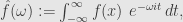
The Laplace transform is given by:

1) $(\mathcal{L}f)(s) = \int_{0^-}^\infty e^{-st}f(t)\,dt$

The Fourier transform is given by:

2) $\hat{f}(\omega) := \int_{-\infty}^{\infty} f(x)\ e^{- \omega i t }\,dt,$

The Two Sided Laplace Transform is given by:

3) $\mathcal{B} \left\{f(t)\right\} = F(s) = \int_{-\infty}^{\infty} e^{-st} f(t) dt.$

Therefor the Fourier transform is the two sided Laplace transform evaluated at $s=i\omega$

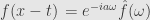
Returning to the one sided Laplace transform:

4) $(\mathcal{L}f)(s) = \int_{a}^b e^{-st}f(t)\,dt= \int_{0^-}^\infty e^{-(\alpha+iw)t}f(t)\,dt$

5) $(\mathcal{L}f)(s) = \int_{a}^b e^{-st}f(t)\,dt= \int_{0^-}^\infty e^{-iw t}f(t)e^{- \alpha t}\,dt$

Integrating by Parts:

Let:

6) $u=e^{- iw t}$
7) $dv=f(t)e^{- \alpha t}\,dt$

8) $V=\int_{a}^tf(t')e^{-\alpha t'}\,dt'=e^{-\alpha t}\int_{t'=a}^tf(t')e^{\alpha (t-t')}\,dt'$

where the low pass filtered version of f(t):

9) $g(t)=f(t)*e^{\alpha t} =e^{-\alpha t} \int_{a}^tf(t')e^{\alpha (t-t')}\,dt'$

and is the convolution of f(t) and the impulse response of a filter (or atleast aproximatly so) with bandwidth $\alpha$ .

Plugging this result into integration by parts gives:

10) $(\mathcal{L}f)(s)=[e^{i \omega t}g(t)]_a^b-\int_a^b-i \omega e^{-i \omega t}e^{-\alpha t}g(t)dt$

or equivalently:

11) $(\mathcal{L}f)(s)=g(b)e^{-i\omega b}-g(a)e^{-i \omega a}+i\int_a^b \omega e^{-i \omega t}e^{-\alpha t}g(t)dt$

The first two terms show how the endpoints chosen effect the transfrom. These two terms will cancel for a given frequency if the distance between the endpoints is some multiple of the period. The last term is the Fouier transform of the smoothed function with the frequencies weighted by $\omega$ and using a windowing function $e^{-\alpha t}$
(note the multiple $i$ is there because the Fourier transform variable $\omega$ is the Laplace transform variable but rotated by 90 degrees.)

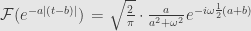
The effect of the windowing function is to smooth the frequency response. This is because multiplication in the time domain is equivalent to convolution in the frequency domain. The following Fourier transform relationship is useful (relationship 205):

12) $\mathcal{F}(e^{- \alpha t} u(t)) \,=\frac{1}{\sqrt{2 \pi} (\alpha + i \omega)}=\frac{1}{\sqrt{2 \pi (\alpha^2 + \omega^2)}}e^{(-i \ tan^{-1}(\alpha,\omega))}$

Note, that if a non causal filter was used for the smoothing the relationship is much simpler.

13) $\mathcal{F}({e}^{-a|t|}) \,=\sqrt{\frac{2}{\pi}} \cdot \frac{a}{a^2 + \omega^2}$

In both cases to properly deal with the end points the time shifting property of the Fourier transform is needed (relationship 102):

14) $f(x - t)\, =e^{- i a \omega} \hat{f}(\omega)\,$

Applying this property to the last two relationships gives:

15) $\mathcal{F}(e^{- \alpha (t-a)} (u(t-a)-u(t-b)) \,=\frac{e^{-ia \omega}-e^{\alpha a-ib\omega}}{\sqrt{2 \pi} (\alpha + i \omega)}$

16) $\mathcal{F}({e}^{-a|(t-b)|}) \,=\sqrt{\frac{2}{\pi}} \cdot \frac{a}{a^2 + \omega^2}e^{-i\omega\frac{1}{2}(a+b)}$

Strictly dealing with the case where a causal filter is used and applying the rule for the Fourier transform of a convolution (Rule 109) we obtain:

17) $(\mathcal{L}f)(s)=g(b)e^{-i\omega b}-g(a)e^{-i \omega a}+i\omega\frac{1}{\sqrt{2\pi}}\mathcal{F}(g(t))*\left( \frac{e^{-ia \omega}-e^{\alpha a-ib\omega}}{\sqrt{2 \pi} (\alpha + i \omega)} \right)$

of equivalently:

18) $\mathcal{L}(f(y))=g(b)e^{-i\omega b}-g(a)e^{-i \omega a}+i\omega\frac{1}{\sqrt{2\pi}}\mathcal{F}(g(t))*\left( \frac{e^{-ia \omega}-e^{\alpha a-ib\omega}}{\sqrt{2 \pi(\alpha^2 +\omega^2)}}e^{ -i tan^{-1}(\alpha,\omega) } \right)$

Some Comments:

1) If $\alpha$ is negative the system is causal, and the filtered version $g(t)$ of the signal $f(t)$ will be causal.

2) Computing the smoothed signal does not save any computations with regards to computing the Laplace transform.

3) The derivation seems to show that their is a relationship between Laplace trancform and a windowed Fouier transform of the filtered signal.

4) To compute the Laplace transform based on the orginal signal use equation (5). To compute it based on the filtered signal use equation (11).

August 30, 2009 - Posted by s243a | Math

8 Comments »

Hmmmmmm………..I forgot about pingbacks, maybe I should only link to other blogs after most of the editing is done.

Comment by s243a | August 30, 2009 | Reply
As a matter of contour integration, if you take the real axis for a Fourier transform, and move it so that the ends fold up along the imaginary axis, but the contour still passes near or below the origin, the result is the difference between two Laplace transforms. Often, because of the effect of a sqrt sign, the two parts ends up being equal and adding.

But I don’t think you’ll find any magic bullet in the FFT, unless you can reverse that contour manoeuvre to get an integral suitable for the purpose.

Comment by Nick Stokes | August 31, 2009 | Reply
- It wasn’t my intent to use the FFT to compute the Laplace transform along the real axis. (However, your idea sounds interesting). Rather, I wish to use the computational efficiency of the FFT to compute the Laplace transform along lines which are parallel to the imaginary axis in Laplace space. Out of the above equations equation (11) is the most suitable for computing this based on the filtered signal and equation (5) is most suitable to compute this based on the original signal.
  
  There is of course a lot of algebra to check here and I was still making corrections after you posted (or at least up to when you posted). The thing that bugs me the most about my derivation is that factor $\omega$ I have as a coefficient for the last term in equation (11). I think this should go away as $\alpha$ approach zero but it doesn’t.
  
  Comment by s243a | August 31, 2009 | Reply
I think my next thread related to this topic will be about compensating for the effects of a finite data set when attempting to evaluate the Laplace transform. The important relationship is the Fourier transform of the unit step function:

$\mathcal{F}(u(x))=\sqrt{\frac{\pi}{2}} \left( \frac{1}{i \pi \omega} + \delta(\omega)\right)$

This relationship may be why I’m getting that factor of $\omega$ in the last term of equation (11)

(Relationship 13)

Comment by s243a | August 31, 2009 | Reply
I know why I didn’t study numerical methods of computing the Laplace transform in school. I didn’t study it because engineers don’t study measure theory :

The meaning of the integral depends on types of functions of interest. For functions that decay at infinity or are of exponential type, it can be understood as a (proper) Lebesgue integral. However, for many applications it is necessary to regard it as a conditionally convergent improper integral at ∞. Still more generally, the integral can be understood in a weak sense, and this is dealt with below.

One can define the Laplace transform of a finite Borel measure μ by the Lebesgue integral[8]

$(\mathcal{L}\mu)(s) = \int_{[0,\infty)} e^{-st}d\mu(t).$

An important special case is where μ is a probability measure or, even more specifically, the Dirac delta function. In operational calculus, the Laplace transform of a measure is often treated as though the measure came from a distribution function ƒ. In that case, to avoid potential confusion, one often writes

$(\mathcal{L}f)(s) = \int_{0^-}^\infty e^{-st}f(t)\,dt$

where the lower limit of 0− is short notation to mean

$\lim_{\varepsilon\to 0^+}\int_{-\varepsilon}^\infty.$

This limit emphasizes that any point mass located at 0 is entirely captured by the Laplace transform. Although with the Lebesgue integral, it is not necessary to take such a limit, it does appear more naturally in connection with the Laplace–Stieltjes transform.,

http://en.wikipedia.org/wiki/Laplace_transform#Fourier_transform

So I guess I have to learn how Lebesque Integration, relates to the Laplace transform.

Comment by s243a | August 31, 2009 | Reply
With regards to my last comment here are some relevent links:

This first link looks pretty complete. I’ll tell you later how easy (or hard) it is to follow for me:
Does there exist the Lebesgue measure in the infinite-dimensional Space

(Last two links are books, so you can’t view the whole book online)
Borel-Laplace Transform and Asymptotic Theory: Introduction to
http://www.worldscibooks.com/etextbook/p245/p245_chap1.pdf

Comment by s243a | August 31, 2009 | Reply
I found a good link for learning mathematics. It is from the university of Colorado.
http://www.uccs.edu/~math/vidarchive.html

The site contains free video’s of the lectures. Apparently the course on real analysis is mostly about measure theory. I found out about it when reading this thread from physics forums.
http://www.physicsforums.com/showthread.php?p=2342489#post2342489

Comment by s243a | September 10, 2009 | Reply
Just posting some old links when I was investigating this stuff further. Haven’t looked at it in a while:

http://www.physicsforums.com/showthread.php?t=334191
http://www.physicsforums.com/showthread.php?t=338132

Comment by s243a | August 19, 2010 | Reply

Earth Cubed

Distributed Climate Science and Computing